3 Excel Formulas that Consultants Must Know

For many years, Excel has been a cornerstone when it comes to analyzing data. Released in 1985, it has grown to the point where every workplace is required to have it. Although Excel can be beneficial in any industry, some people dread the sight of a blank spreadsheet.

To help you combat your Excel anxiety, below are 3 important formulas that will help to transform you into a pro user.

1. VLOOKUP

Vlookup (short for Vertical Lookup) is one of the best formulas in Excel’s arsenal. It is designed to work with data organized in columns.

The syntax of the formula is as follows:

=VLOOKUP(lookup_value, table_array, col_index_num, [range_lookup])

1. lookup_value – The value you want to lookup
2. table_array – The range where the lookup value is located. Note that the lookup value MUST be in the first column in the selected range.
3. col_index_num – The number of the column for the return value in the range previously specified. Suppose the range is C2:G25. Column C is counted as the first column, D is the second column, E is the third, and so on.
4. [range_lookup] – Here you can specify if you want an exact match (denoted as FALSE) or an approximate match (denoted as TRUE).

VLOOKUP Example

Imagine there is a company which keeps an hourly rate spreadsheet for employees (see “Hourly Rate” below) and a sales team salary spreadsheet (see “Sales Team Salary” below). If we want to get the Hourly Rate for each employee listed in Sales Team Salary, we can use VLOOKUP.

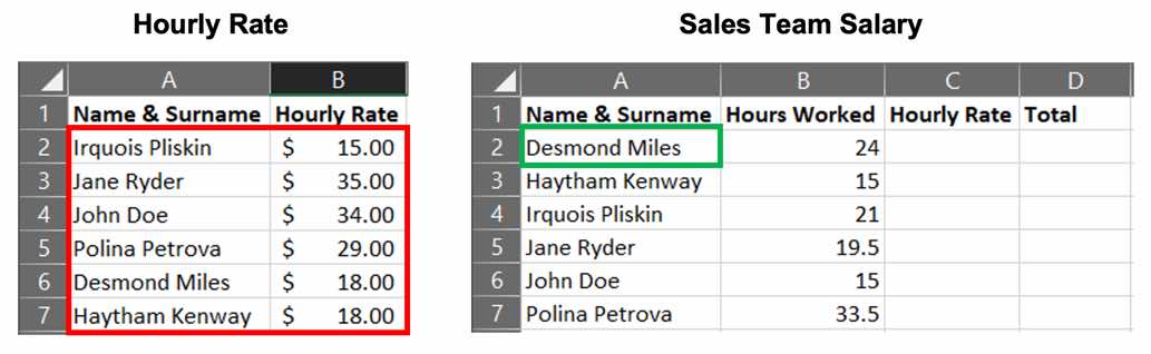
The VLOOKUP formula is entered in cell C2 of the Sales Team Salary table and dragged down. The way we select each item of the syntax is detailed below:

=VLOOKUP(lookup_value, table_array, col_index_num, [range_lookup])

For col_index_num we write 2 because the return value is in the second column, and for [range_lookup] we select FALSE so it gives us an exact match.

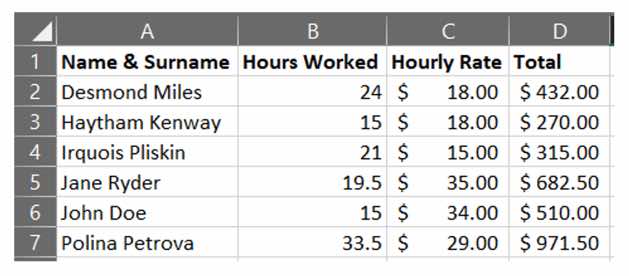
The result in the Sales Team Salary table will be as follows:

2. SUMIFS

Sumifs is another powerful Excel function that sums up the values based on one or more criteria and returns a numeric value.

The syntax of the formula is as follows:

=SUMIFS(sum_range, criteria_range1, criteria1, [criteria_range2, criteria2], …)

1. sum_range – The range of cells to sum
2. criteria_range1 – The range of cells which you want to apply criteria1 against
3. criteria1 – A criterion that is applied against criteria_range1 in order to determine which cells to add
4. criteria_range2 – The range of cells which you want to apply criteria2 against
5. criteria2 – A criterion that is applied against criteria_range2 in order to determine which cells to add

SUMIFS Example

Imagine there is a company that runs a theme park and keeps a record of the number of visitors on different dates (as seen in the table below). If we want to find the total number of visitors between January 1^st and February 28^th, we can use SUMIFS.

The SUMIFS formula is entered into cell D5. The way we select each item of the syntax is detailed below:

=SUMIFS(sum_range, criteria_range1, criteria1, [criteria_range2, criteria2], …)

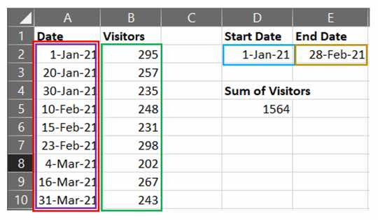
Note that for criteria1 and criteria2 you should input “>=”&D2 and “<=”&E2 respectively. This tells the SUMIFS formula to sum the number of visitors between the specified dates.

3. CONCATENATE

Concatenate is a well-known formula in Excel which joins together the contents of two or more cells into a single cell.

The syntax for the formula is as follows:

=CONCATENATE(text1, [text2],…)

1. text1 – The first item that will be joined to subsequent items. This can be a number, value, or cell reference.
2. [text2] – The second item that will be joined to the first one. This can be a number, value, or cell reference.

CONCATENATE Example

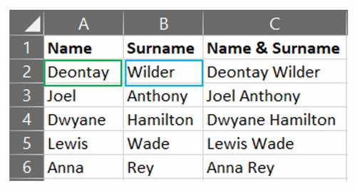
Imagine that the company has a list of names and surnames separated into two different columns (columns A & B) and wants to join them together in column C (as seen in the table below).

The CONCATENATE formula is entered in cell C2 and dragged down. The way we select each item of the syntax is detailed below:

=CONCATENATE(text1, [text2], [text3])

Note that for [text2] you input only “ “ which denotes to Excel that you are including a blank space in the formula.

Final thoughts

Excel is a must-use tool for consultants and data analysts alike.

The 3 formulas detailed in this article will help to make even the most novice of users feel like a pro, and build a solid foundation that will allow you to advance into more complex formulas.

Loredan Emini graduated from Rochester Institute of Technology in Economics & Management. He currently works as a Power BI specialist for a German company, and as a lecturer of Power BI.

Image: Pixabay

🔴 Interested in consulting?

🔴 Interested in consulting?

Follow now on LinkedIn.