
This is a continuation of Part 1 where different types and benefits of customer segmentation were introduced.
In this article we will focus on three customer segmentation methods that use statistical techniques: cluster analysis (K-Means), cluster analysis (Latent Class Analysis), and Tree analysis (CHAID).
Let’s first define a problem and see how each method approaches it.
The Question
The Head of Retail Banking at a big bank has a large database of branch customers like financial information (e.g. Branch ID, Customer ID, Account ID, Product ID, open date, close date, and deposit balances) and demographic information (e.g. age, gender, education, employment, annual income, home ownership, and residency). He wants to understand the different customer segments to tailor the next marketing strategy.
The Analytical Methods
1. Cluster Analysis (K-Means)
The main idea of cluster analysis is to identify groupings of objects (customers) that are similar with respect to a collection of characteristics (financial and demographic information) and are as dissimilar as possible from an adjacent grouping of objects. The number of clusters (segments) is dependent upon the type of algorithm used to identify the clusters. The characteristics can be a set of data elements (variables) that describe each customer.
Within a cluster analysis, one widely used methodology is K-Means Clustering, where K represents the number of clusters to be created. Each cluster is centered around a particular point called a centroid.

The above image represents K-Means clustering where K=3. Each individual dot represents a single customer and it has formed three segments around three centroids. The centroid is made up from the average values of the data elements making up the clusters.
A customer is assigned to a segment by calculating a distance measurement to each of the centroids. The score is commonly calculated from the Euclidean distance. The Euclidean distance between points a and b is the length of the line connecting them $latex (\bar{ab}) $, which is calculated using the formula:
$latex d(a,b) = \sqrt{\sum_{i=0}^{n}(a_{i} – b_{i})^{2}} $
Where n represents the number of dimensions (variables), where n=2 in this case. It can be looking at the annual income (x-axis) and deposit balance (y-axis). So if $latex a = (a_{1}, a_{2}) $ and $latex b = (b_{1}, b_{2}) $ then the distance is given by $latex d(a, b) = \sqrt{(a_{1} – b_{1})^{2}+(a_{2} – b_{2})^{2}} $. In a typical business scenario, there could be several variables (e.g. product, age, residency) which could possibly generate much more realistic and business-specific insights.
The centroid with the closest distance becomes the customer’s home segment. The objective of any clustering algorithm is to ensure that the distance between data points in a cluster is very low compared to the distance between two clusters. In other words, customers of a segment are very similar, and customers of different segments are extremely dissimilar.
There’s often a great deal of subjectivity associated with cluster analysis with the number of clusters being determined based upon the usability and usefulness of the corresponding groupings. The final clusters are often given names that summarise their key traits, such as “young, educated, high-income earner”.
2. Cluster Analysis (Latent Class Analysis)
Latent class analysis (LCA) involves the construction of “Latent Classes” which are unobserved (latent) clusters (segments). This method uses probability modeling to describe the distribution of the data (i.e. maximize the overall fit of the model to the data). So instead of finding clusters with some arbitrary chosen distance measure, you use a model that describes distribution of your data and based on this model you assess probabilities that certain cases are members of certain latent classes (segments).
So, you could say that LCA is a top-down approach (you start by describing the distribution of your data), while K-Means is a relatively bottom-up approach (you find similarities between cases). The model can identify patterns in multiple dependent variables (e.g. products held) and quantify correlation of dependent variables with related variables (e.g. deposit balances). For each customer, the analysis delivers a probability of belonging to each cluster. Customers are assigned to the cluster to which they have the highest probability of belonging.
In summary, LCA has three main differences from K-Means clustering:
- LCA uses probabilities, instead of distances, to classify cases into segments.
- Variables may be continuous, categorical (nominal or ordinal), or counts or any combination of these.
- LCA can include respondents who have missing values for some of the dependent variables, which reduces the rate of misclassification (assigning consumers to the wrong segment).
Despite these benefits, LCA has a few drawbacks. For one thing, K-Means is much faster to compute which means K-Means can be a preferable method when dealing with a huge database. Additionally, LCA requires advanced knowledge of statistics to wade through the myriad of options available. Lastly, because LCA can handle so many variables it is tempting to add more segmentation inputs than are really necessary. Undue complexity makes interpreting the segmentation solution more difficult.
3. Tree Analysis (CHAID)
Tree Analysis starts with partitioning each object (customer) into one of two outcomes (this is the dependent variable). Examples include response to a marketing promotion (0=No, 1=Yes), opening a specific product (chequing, savings) or making a repeat deposit. This is the starting point for the tree.
Other characteristics (the independent variables) are used to further partition customers. Each partition creates a new branch of the tree. For example, customers who responded to a marketing promotion might be significantly more likely to fall within a specific age range (say, age 24 to 30) compared to customers who did not respond.
Further analysis might show that customers age 24 to 30, living in urban markets, who do not have any children living at home, are even more likely to respond. This creates a new branch of the tree (perhaps called “Childless Metro Millennials”). The branching process continues until there are no more statistically significant partitions that can be made. Each ending branch (called a node) represents a customer segment. The number of final nodes depends on how well the independent variables are able to differentiate the behavior under study.
One of the oldest tree classification methods is CHAID, which stands for Chi-squared Automatic Interaction Detector. CHAID can be used to “build” non-binary trees (i.e. trees where more than two branches can attach to a single root or node), based on a relatively simple algorithm that is particularly well suited for the analysis of large datasets.
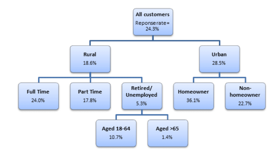
The above illustrates an example of a CHAID tree diagram showing the response rates for a direct marketing campaign for different subsets of customers. Chi-square tests are applied at each of the stages in building the CHAID tree to ensure that each branch is associated with a statistically significant predictor of the response variable (e.g. response rate).
In CHAID analysis, if the dependent variable is continuous (e.g. sales recorded in $’s), the F test is used and if the dependent variable is categorical, the chi-squared test is used.
- A chi-squared test of independence examines the relationship between two nominal variables. It examines the cell counts of each combination of variable and compares the count with the expected value for that cell. The expected value is the value that cell would be if no relationship occurred between the variables. If significance is found, then there was a significant difference between the observed counts and the expected values.
- $latex \chi_{c}^{2} $: The chi-square test statistic; used with the $latex df $ (subscript “c”) to compute the p-value
- $latex df $ (degrees of freedom): Determined by (number of rows – 1) x (number of columns – 1)
- $latex p $ (probability value): Gives the probability of obtaining the observed results if the null hypothesis is true; in most cases a result is considered statistically significant if p ≤ 0.05.
Each pair of predictor categories are assessed to determine what is least significantly different with respect to the dependent variable. When testing with a 5% significance level (i.e. considering a p-value of less than 0.05 to be statistically significant) we have a one in 20 chance of finding a false-positive result; concluding that there is a difference when in fact none exists. The more tests that we do, the greater the chance we will find one of these false-positive results (inflating the so-called Type I error), so adjustments to the p-values are used to counter this, so that stronger evidence is required to indicate a significant result.
Generally, a large sample size is needed to perform a CHAID analysis. At each branch, we reduce the number of observations available as we split the total population. So with a small total sample size the individual groups can quickly become too small for reliable analysis.
Leverage tools for computation
As you can probably imagine, the computations for all three methods can get extremely lengthy and tedious. You’ll probably want to use technology. For a basic exploratory analysis many choose to use the statistical tools in Excel. Not only is it readily available as part of MS Office, but its spreadsheet functionality means that most users find it easy to use. However, it is important to recognize that there are a number of drawbacks to using Excel; its data analysis tools are limited and there is very little flexibility over the methods used and the output given.
Fortunately, there are more sophisticated tools available, such as Python, SPSS, and R. Thanks to the internet there are numerous free courses that are easily accessible to get you up to speed. Try starting a side project of your interest using these tools – it’s the best way to learn.
Jason Oh is a Senior Consultant, Strategy & Customer at EY with project experiences in commercial due diligence and corporate strategy planning. Previously, he was a Management Consultant at Novantas with a focus on the financial services sector, where he advised on pricing, marketing, channel distribution, digital transformation and due diligence.
Image: Pexels